Compare gaussian copula and vine copula
Introduction
In this example, we will show the differences between using Gaussian copula and vine copula when simulate new data. Vine copula can better estimate the high-dimensional gene-gene correlation, however, the simulation with vine copula does takes more time than with Gaussian copula. If your reference dataset have more than 1000 genes, we recommend you simulate data with Gaussian copula.
Import packages and Read in data
import pacakges
import re
import anndata as ad
import numpy as np
import pandas as pd
import scanpy as sc
import scDesign3Py
Read in data
The raw data is from the R package DuoClustering2018 and converted to .h5ad file using the R package sceasy.
data = ad.read_h5ad("data/Zhengmix4eq.h5ad")
data.obs["cell_type"] = data.obs["phenoid"]
data.var.index = data.var["symbol"]
data.layers["log"] = data.X.copy()
sc.pp.normalize_total(data,target_sum=1e4,layer="log")
sc.pp.log1p(data,layer="log")
For demonstration purpose, we use the top 100 highly variable genes. We further filtered out some highly expressed housekeeping genes and added TF genes.
humantfs = pd.read_csv("http://humantfs.ccbr.utoronto.ca/download/v_1.01/TF_names_v_1.01.txt",header=None)
# choose HVG genes
sc.pp.highly_variable_genes(data,layer="log",n_top_genes=100)
gene_list = data.var[data.var["highly_variable"] == True].index.to_series()
# get whole candidate genes
gene_list = pd.unique(pd.concat([humantfs[0],gene_list]))
# filter out unneeded genes
gene_list = [x for x in gene_list if (re.match("RP",x) is None) and (re.match("TMSB",x) is None) and (not x in ["B2M", "MALAT1", "ACTB", "ACTG1", "GAPDH", "FTL", "FTH1"])]
# get final data
subdata =  data[:,list(set(gene_list).intersection(set(data.var_names)))]
subdata
View of AnnData object with n_obs × n_vars = 3555 × 138
    obs: 'barcode', 'phenoid', 'total_features', 'log10_total_features', 'total_counts', 'log10_total_counts', 'pct_counts_top_50_features', 'pct_counts_top_100_features', 'pct_counts_top_200_features', 'pct_counts_top_500_features', 'sizeFactor', 'cell_type'
    var: 'id', 'symbol', 'mean_counts', 'log10_mean_counts', 'rank_counts', 'n_cells_counts', 'pct_dropout_counts', 'total_counts', 'log10_total_counts', 'highly_variable', 'means', 'dispersions', 'dispersions_norm'
    uns: 'log1p', 'hvg'
    obsm: 'X_pca', 'X_tsne'
    layers: 'logcounts', 'normcounts', 'log'
Simulation
We then use scDesign3Py to simulate two new datasets using Gaussian copula and vine copula respectively.
gaussian = scDesign3Py.scDesign3(n_cores=3,parallelization="pbmcmapply")
gaussian.set_r_random_seed(123)

gaussian_res = gaussian.scdesign3(anndata = subdata,
                            celltype = 'cell_type',
                            corr_formula = "cell_type",
                            mu_formula = "cell_type",
                            sigma_formula = "cell_type",
                            copula = "gaussian",
                            assay_use = "normcounts",
                            family_use = "nb",
                            usebam=False,
                            pseudo_obs = True,
                            return_model = True)
vine = scDesign3Py.scDesign3(n_cores=3,parallelization="pbmcmapply")
vine.set_r_random_seed(123)

vine_res = vine.scdesign3(anndata = subdata,
                        celltype = 'cell_type',
                        corr_formula = "cell_type",
                        mu_formula = "cell_type",
                        sigma_formula = "cell_type",
                        copula = "vine",
                        assay_use = "normcounts",
                        family_use = "nb",
                        usebam=False,
                        pseudo_obs = True,
                        return_model = True)
Visualization
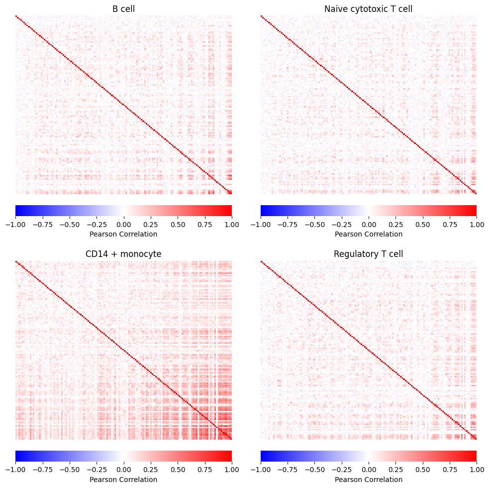
For the simulation result using Gaussian copula, the return object contains a corr_list which is the gene-gene correlation matrices for each group that user specified, in this case, the groups are cell types. For the simulation result using vine copula, the corr_list gives the vine structure for each group that user specified, in this case, the groups are cell types. We then reformat the two corr_list and visualize them.
import matplotlib.pyplot as plt
import networkx as nx
import seaborn as sns
name_dic = {
    "b.cells": "B cell",
    "naive.cytotoxic": "Naive cytotoxic T cell",
    "cd14.monocytes": "CD14 + monocyte",
    "regulatory.t": "Regulatory T cell",
}
Gaussian copula
Show code cell source
# pre-process
gaussian_corr = gaussian_res["corr_list"]
heatmap_order = subdata.var.sort_values("mean_counts").index.to_list()
gaussian_corr = {name_dic[k]:v.loc[heatmap_order,heatmap_order] for k,v in gaussian_corr.items()}

# start to plot
fig_gau, axes_gau = plt.subplots(2, 2, figsize=(2 * 5, 2 * 5))
fig_gau.tight_layout()
for i, (group, data) in enumerate(gaussian_corr.items()):
    row, col = np.unravel_index(i, axes_gau.shape)
    ax = axes_gau[row, col]
    sns.heatmap(
        data=data,
        vmin=-1,
        vmax=1,
        cmap="bwr",
        cbar_kws={
            "label": "Pearson Correlation",
            "orientation": "horizontal",
            "pad": 0.05,
        },
        xticklabels=[],
        yticklabels=[],
        ax=ax,
    )
    ax.set_title(group)
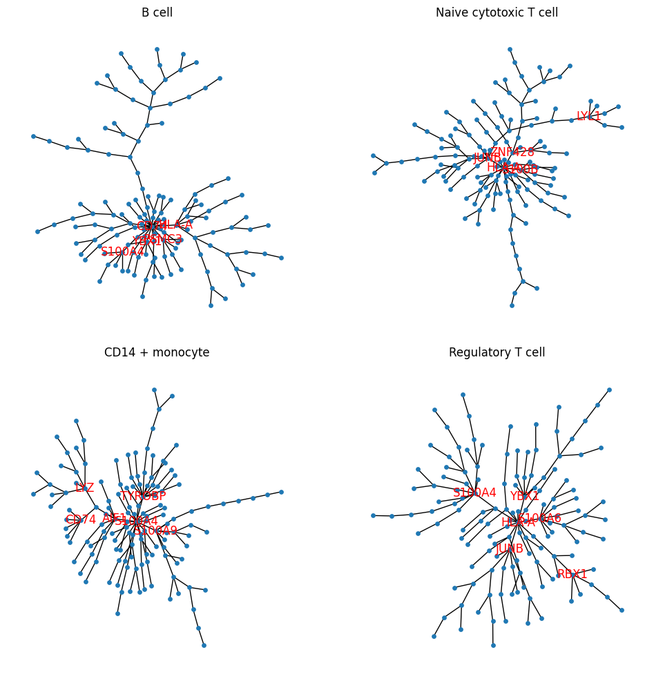
Vine copula
Comparing with the visualization above, the plots below give more direct visualization about which genes are connected in the vine structure and show gene networks.
Show code cell source
vine_corr = vine_res["corr_list"]

def get_adjacency_matrix(input):
    structure = input["structure"]
    order = structure["order"].astype("int")
    d = int(structure["d"][0])
    trunc_lvl = int(structure["trunc_lvl"][0])
    m = np.zeros((d,d),dtype=int)
    m[np.diag_indices_from(m)] = order
    for i in range(m.shape[0]):
        m[:,i] = np.flipud(m[:,i])
    for i in range(min(trunc_lvl,d-1)):
        newrow = order[structure["struct_array"].byindex(i)[-1].astype("int")-1]
        m[i,0:len(newrow)] = newrow
    I = np.zeros((d,d),dtype=int)
    E = np.array([m[[d-i-1,0],i] for i in range(d-1)])
    for i in range(len(E)):
        index = np.where(np.isin(order,E[i,:]))[0]
        I[index[0],index[1]] = I[index[1],index[0]] = 1
    name = np.array(input["names"])
    name = name[order-1]
    res = pd.DataFrame(I,index=name,columns=name)
    return res

# plot
degree_thresh = 4

fig_vine, axes_vine = plt.subplots(2, 2, figsize=(2 * 5, 2 * 5))
fig_vine.tight_layout()
for i, (group, data) in enumerate(vine_corr.items()):
    row, col = np.unravel_index(i, axes_vine.shape)
    ax = axes_vine[row, col]
    adjacency_matrix = get_adjacency_matrix(data)
    G = nx.from_pandas_adjacency(adjacency_matrix, create_using=nx.Graph())
    pos = nx.kamada_kawai_layout(G, scale=3)
    nx.draw_networkx(
        G,
        pos=pos,
        node_size=15,
        with_labels=True,
        ax=ax,
        labels={n: n if G.degree[n] > degree_thresh else "" for n in G.nodes},
        font_color = "red",
    )
    ax.set_title(name_dic[group])
    ax.axis("off")