Quick Start
Introduction
The R package scDesign3 is a unified probabilistic framework that generates realistic in silico high-dimensional single-cell omics data of various cell states, including discrete cell types, continuous trajectories, and spatial locations by learning from real datasets. scDesign3Py is the python interface for scDesign3.
As a quick start, we demonstrate how to use scDesign3Py to simulate an scRNA-seq dataset with one continuous developmental trajectory.
Step 1: Import packages and Read in data
import pacakges
import anndata as ad
import numpy as np
import scDesign3Py
Read in data
The raw data is from the scvelo, which describes pancreatic endocrinogenesis. We pre-select the top 1000 highly variable genes and filter out some cell types to ensure a single trajectory.
To save time, we only use the top 30 genes.
data = ad.read_h5ad("data/PANCREAS.h5ad")
data = data[:, 0:30]
data
View of AnnData object with n_obs × n_vars = 2087 × 30
    obs: 'clusters_coarse', 'clusters', 'S_score', 'G2M_score', 'cell_type', 'sizeFactor', 'pseudotime'
    var: 'highly_variable_genes'
    obsm: 'X_pca', 'X_umap', 'X_x_pca', 'X_x_umap'
Step 2: scdesign3() performs all-in-one simulation
First create an instance of the scDesign class to use the scdesign3() method, when creating the instance, we can also set up the basic settings when initializing.
Note
If you are a windows user, please refer to Get BPPARAM section to use more than one core for parallel computing.
test = scDesign3Py.scDesign3(n_cores=3, parallelization="pbmcmapply")
test.set_r_random_seed(123)
The function scdesign3() takes in an anndata.AnnData object with the cell covariates (such as cell types, pesudotime, or spatial coordinates) stored in the anndata.AnnData.obs, and performs the all-in-one simulation.
simu_res = test.scdesign3(
    anndata=data,
    default_assay_name="counts",
    celltype="cell_type",
    pseudotime="pseudotime",
    mu_formula="s(pseudotime, k = 10, bs = 'cr')",
    sigma_formula="s(pseudotime, k = 5, bs = 'cr')",
    family_use="nb",
    usebam=False,
    corr_formula="1",
    copula="gaussian",
)
Note
Details of creating the instance of the scDesign3 class and the usage of the scdesign3() function will be shown in tutorial section.
Step 3: Construct new anndata.AnnData object with the simulated result
Besides constructing the simulated anndata.AnnData object, we can also calculate the log transformed data for visualization.
simu_data = ad.AnnData(X=simu_res["new_count"], obs=simu_res["new_covariate"])
simu_data.layers["log_transformed"] = np.log1p(simu_data.X)
data.layers["log_transformed"] = np.log1p(data.X)
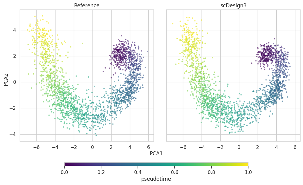
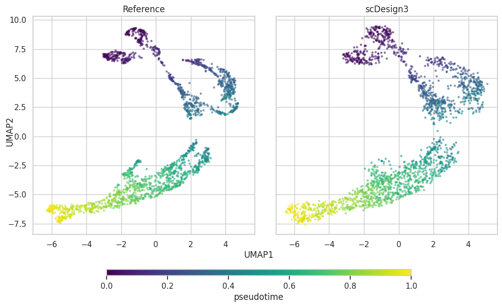
Step 4: Visualization
Note
Details of the plot process will be shown in tutorial section.
plot = scDesign3Py.plot_reduceddim(
    ref_anndata=data,
    anndata_list=simu_data,
    name_list=["Reference", "scDesign3"],
    assay_use="log_transformed",
    if_plot=True,
    color_by="pseudotime",
    n_pc=20,
    point_size=5,
)
UMAP plot
plot["p_umap"]
PCA plot
plot["p_pca"]