Extension: mcRigor two-step

#tools::R_user_dir("mcRigor", which="cache")
library(mcRigor)
library(Seurat)
library(ggplot2)

Introduction

Overview

In this tutorial, we demonstrate how to use the mcRigor two-step extension of mcRigor to further dissect previously identified dubious metacells and reorganize their constituent cells into more trustworthy metacells. We will apply mcRigor two-step to a semi-synthetic single-cell RNA sequencing (scRNA-seq) dataset with known ground-truth metacell trustworthiness.

As its name suggests, mcRigor two-step operates in two consecutive steps:

Step 1 (function mcRigorTS_Step1): Identify the single cells that constitute dubious metacells and need to be re-partitioned.
Step 2 (function mcRigorTS_Step2): Re-partition the identified single cells under the optimized granularity level and output the final metacell partition.

Input preparation

As for the main functionalities of mcRigor, we also work on two main inputs in mcRigor two-step: 1. the raw scRNA-seq data and 2. candidate metacell partitions generated by either existing metacell partitioning methods or ad hoc approaches. The raw scRNA-seq data needs to be provided as a Seurat object, obj_singlecell. The semi-synthetic scRNA-seq data, whose generation process is described in Liu and Li, 2024, stored as a rds file syn.rds, is available with the mcRigor package as an example. The metacell partitions should be provided as a dataframe, cell_membership, showing the assignment of single cells to metacells in each partition. Specifically, each column of this dataframe should represent the matacell partition corresponding to one granularity level and each row of the dataframe should represent one single cell. Note that we require the column namse of the dataframe to be set as the granularity level values in the character type. The metacell partitions for the semi-synthetic scRNA-seq data generated by the SEACells method (Persad et al., 2023), stored as a csv file seacells_cell_membership_rna_syn.csv, is available with the mcRigor package as an example. This csv file contains series of metacell partitions, which were generated under different granularity levels. Note that granularity level, $\gamma$ , is a key parameter for metacell partitioning and is defined as the ratio of the number of single cells to the number of metacells. We first load these inputs:

sc_dir = system.file('extdata', 'syn.rds', package = 'mcRigor')
obj_singlecell= readRDS(file = sc_dir)

membership_dir = system.file('extdata', 'seacells_cell_membership_rna_syn.csv', package = 'mcRigor')
cell_membership <- read.csv(file = membership_dir, check.names = F, row.names = 1)

Step 1: identify single cells that constitute the dubious metacells

In this tutorial, we focus on the metacell partition corresponding to the granularity level $\gamma = 50$ , specified by tgamma = 50. We first run the main mcRigor function mcRigor_DETECT to check whether this partition contains any dubious metacells. If no dubious metacells are detected, there is no need to apply mcRigor two-step.

tgamma = 50
detect_res = mcRigor_DETECT(obj_singlecell = obj_singlecell, cell_membership = cell_membership, tgamma = tgamma)

table(detect_res$mc_res)
#> 
#>     dubious trustworthy 
#>          28         240

We proceed with mcRigor two-step because dubious metacells exist in this partition We call the function mcRigorTS_Step1 to identify the single cells that constitute dubious metacells (under a lower divergence score threshold) and need to be re-partitioned. Note that we input the permutation results, detect_res$TabMC, obtained from the previous code block to save computation time here, although it is also acceptable to leave this argument as its default value (NULL). We need to specify the metacell partitioning method (e.g., SEACells, MetaCell, MetaCell2, SuperCell, or MetaQ) by setting the argument method, ensuring that the function generates outputs in the correct format.

sc_membership = cell_membership[[as.character(tgamma)]]
names(sc_membership) = rownames(cell_membership)

step1_res = mcRigorTS_Step1(obj_singlecell = obj_singlecell, sc_membership = sc_membership, TabMC = detect_res$TabMC, method = 'seacells')
#> Testing thresholds (Thre) not provided. Calculating thresholds with defaults...

The Seurat object of single cells that need to be re-partitioned is stored in the obj_sc_dub field of the output step1_res. If the metacell partitioning method used is SEACells, MetaCell2, or MetaQ,, mcRigorTS_Step1 will automatically generate two CSV files (counts.csv and metadata.csv) in the current working directory. These files can be directly used as input for the corresponding metacell partitioning methods in Python.

step1_res$obj_sc_dub
#> An object of class Seurat 
#> 1982 features across 2883 samples within 1 assay 
#> Active assay: RNA (1982 features, 1982 variable features)
#>  3 layers present: counts, data, scale.data
#>  2 dimensional reductions calculated: pca, umap
list.files("seacells/")
#> [1] "counts.csv"   "metadata.csv"

Step 2: Re-organize the single cells into more trustworthy metacells

We then need to apply the chosen metacell partitioning method (e.g., SEACells, MetaCell, MetaCell2, SuperCell, MetaQ) to these identified single cells to obtain more trustworthy metacell partitions for them, under granularity level smaller than tgamma (recommend obtaining all the candidate paritions corresponding to granularity levels from 2 to tgamma-1). One can refer to the Implementing metacell partitioning methods tutorial for more guidnance on how to obtain the metacell partitions. The candidate metacell partitions can be stored in csv file and read into an R object cell_membership_twostep using cell_membership_twostep <- read.csv(file = "/path/to/the/csv/file", check.names = F, row.names = 1). For illustration purpose in this tutorial, we set cell_membership_twostep as the partitions corresponding to small granularity levels in cell_membership_all.

cell_membership_twostep = cell_membership[ , as.numeric(names(cell_membership)) < 50]
cell_membership_twostep = cell_membership_twostep[colnames(step1_res$obj_sc_dub),]

We call the function mcRigorTS_Step2 to select the optimal granularity level and output the final metacell partition with remaining dubious metacells flagged.

step2_res = mcRigorTS_Step2(step1_res = step1_res, obj_singlecell = obj_singlecell, cell_membership_twostep = cell_membership_twostep)
#> Names of identity class contain underscores ('_'), replacing with dashes ('-')
#> First group.by variable `Metacell` starts with a number, appending `g` to ensure valid variable names
#> This message is displayed once every 8 hours.

The Seurat object of the final metacells are stored in the obj_metacell_final field of the output step2_res with the dubious metacell detection results recorded in its metadata under the name mcRigor. Another field, obj_metacell_final_withsc, is the Seurat object of the final metacells where all dubious metacells have been dissected into their constituent single cells (i.e., no dubious metacells remain). Users can choose which object to use depending on their analytical needs. In addtion, the output step2_res includes two visualization fields: plot and plot_withsc, which correspond to UMAP plots of single cells with obj_metacell_final and obj_metacell_final_withsc metacells projected onto the UMAP space, respectively.

step2_res$obj_metacell_final
#> An object of class Seurat 
#> 2000 features across 311 samples within 1 assay 
#> Active assay: RNA (2000 features, 0 variable features)
#>  2 layers present: counts, data
step2_res$plot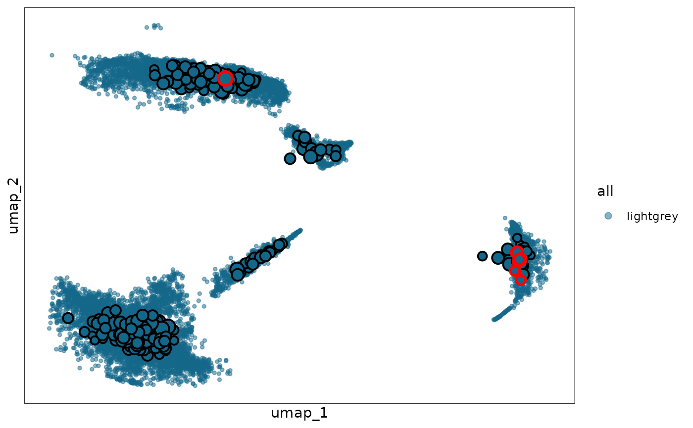

Session information

sessionInfo()
#> R version 4.5.1 (2025-06-13)
#> Platform: x86_64-pc-linux-gnu
#> Running under: Ubuntu 24.04.3 LTS
#> 
#> Matrix products: default
#> BLAS:   /usr/lib/x86_64-linux-gnu/openblas-pthread/libblas.so.3 
#> LAPACK: /usr/lib/x86_64-linux-gnu/openblas-pthread/libopenblasp-r0.3.26.so;  LAPACK version 3.12.0
#> 
#> locale:
#>  [1] LC_CTYPE=C.UTF-8       LC_NUMERIC=C           LC_TIME=C.UTF-8       
#>  [4] LC_COLLATE=C.UTF-8     LC_MONETARY=C.UTF-8    LC_MESSAGES=C.UTF-8   
#>  [7] LC_PAPER=C.UTF-8       LC_NAME=C              LC_ADDRESS=C          
#> [10] LC_TELEPHONE=C         LC_MEASUREMENT=C.UTF-8 LC_IDENTIFICATION=C   
#> 
#> time zone: UTC
#> tzcode source: system (glibc)
#> 
#> attached base packages:
#> [1] stats     graphics  grDevices utils     datasets  methods   base     
#> 
#> other attached packages:
#> [1] ggplot2_4.0.0      Seurat_5.3.0       SeuratObject_5.2.0 sp_2.2-0          
#> [5] mcRigor_1.0        BiocStyle_2.36.0  
#> 
#> loaded via a namespace (and not attached):
#>   [1] deldir_2.0-4           pbapply_1.7-4          gridExtra_2.3         
#>   [4] rlang_1.1.6            magrittr_2.0.4         RcppAnnoy_0.0.22      
#>   [7] spatstat.geom_3.6-0    matrixStats_1.5.0      ggridges_0.5.7        
#>  [10] compiler_4.5.1         reshape2_1.4.4         png_0.1-8             
#>  [13] systemfonts_1.3.1      vctrs_0.6.5            stringr_1.5.2         
#>  [16] pkgconfig_2.0.3        fastmap_1.2.0          labeling_0.4.3        
#>  [19] promises_1.3.3         rmarkdown_2.30         ragg_1.5.0            
#>  [22] purrr_1.1.0            xfun_0.53              cachem_1.1.0          
#>  [25] jsonlite_2.0.0         goftest_1.2-3          later_1.4.4           
#>  [28] spatstat.utils_3.2-0   irlba_2.3.5.1          parallel_4.5.1        
#>  [31] cluster_2.1.8.1        R6_2.6.1               ica_1.0-3             
#>  [34] spatstat.data_3.1-8    stringi_1.8.7          bslib_0.9.0           
#>  [37] RColorBrewer_1.1-3     reticulate_1.43.0      spatstat.univar_3.1-4 
#>  [40] parallelly_1.45.1      lmtest_0.9-40          jquerylib_0.1.4       
#>  [43] scattermore_1.2        Rcpp_1.1.0             bookdown_0.45         
#>  [46] knitr_1.50             tensor_1.5.1           future.apply_1.20.0   
#>  [49] zoo_1.8-14             sctransform_0.4.2      httpuv_1.6.16         
#>  [52] Matrix_1.7-3           splines_4.5.1          igraph_2.2.0          
#>  [55] tidyselect_1.2.1       abind_1.4-8            yaml_2.3.10           
#>  [58] spatstat.random_3.4-2  spatstat.explore_3.5-3 codetools_0.2-20      
#>  [61] miniUI_0.1.2           listenv_0.9.1          plyr_1.8.9            
#>  [64] lattice_0.22-7         tibble_3.3.0           withr_3.0.2           
#>  [67] shiny_1.11.1           S7_0.2.0               ROCR_1.0-11           
#>  [70] evaluate_1.0.5         Rtsne_0.17             future_1.67.0         
#>  [73] fastDummies_1.7.5      desc_1.4.3             survival_3.8-3        
#>  [76] polyclip_1.10-7        fitdistrplus_1.2-4     pillar_1.11.1         
#>  [79] BiocManager_1.30.26    KernSmooth_2.23-26     plotly_4.11.0         
#>  [82] generics_0.1.4         RcppHNSW_0.6.0         scales_1.4.0          
#>  [85] globals_0.18.0         xtable_1.8-4           glue_1.8.0            
#>  [88] lazyeval_0.2.2         tools_4.5.1            data.table_1.17.8     
#>  [91] RSpectra_0.16-2        RANN_2.6.2             fs_1.6.6              
#>  [94] dotCall64_1.2          cowplot_1.2.0          grid_4.5.1            
#>  [97] tidyr_1.3.1            nlme_3.1-168           patchwork_1.3.2       
#> [100] cli_3.6.5              spatstat.sparse_3.1-0  textshaping_1.0.4     
#> [103] spam_2.11-1            viridisLite_0.4.2      dplyr_1.1.4           
#> [106] uwot_0.2.3             gtable_0.3.6           sass_0.4.10           
#> [109] digest_0.6.37          progressr_0.17.0       ggrepel_0.9.6         
#> [112] htmlwidgets_1.6.4      farver_2.1.2           htmltools_0.5.8.1     
#> [115] pkgdown_2.1.3          lifecycle_1.0.4        httr_1.4.7            
#> [118] mime_0.13              MASS_7.3-65