Evaluate clustering goodness-of-fit

Introduction

In this example, we will show how to use scDesign3Py to evaluate the clustering goodness-of-fit for different cell-type assignments. If the true labels are unavailable and we have little prior knowledge, the scDesign3Py BIC can serve as an unsupervised metric.

Import packages and Read in data

import pacakges

import anndata as ad
import pandas as pd
import scanpy as sc
import scDesign3Py

from sklearn.metrics import adjusted_rand_score

Read in data

The raw data is from the R package DuoClustering2018 and converted to .h5ad file using the R package sceasy.

The cluster result is also got from the R package DuoClustering2018 as the package has already provided various clustering results.

data = ad.read_h5ad("data/Zhengmix4eq.h5ad")
cluster_res = pd.read_csv("data/clusterres_Zhengmix4eq.csv",index_col=0)
cluster_res = cluster_res[cluster_res["method"].isin(["PCAKmeans"]) & (cluster_res["run"] == 1)]

For demonstration purpose, we use the Zhengmix4eq dataset in the package with top 30 highly variable genes and the corresponding k-means clustering results with \(k = 2 \sim 10\).

kmeans_res = cluster_res.groupby("k")
ncell = data.n_obs
ngene = 30
ntrain = int(ncell/5)

# choose HVG genes
data.layers["log"] = data.X.copy()
sc.pp.normalize_total(data,target_sum=1e4,layer="log")
sc.pp.log1p(data,layer="log")
sc.pp.highly_variable_genes(data,layer="log",n_top_genes=ngene)
data = data[:,data.var["highly_variable"] == True]

train_data = data[data.obs.sample(n=ntrain,random_state=123).index,:]
train_data

View of AnnData object with n_obs × n_vars = 711 × 30
    obs: 'barcode', 'phenoid', 'total_features', 'log10_total_features', 'total_counts', 'log10_total_counts', 'pct_counts_top_50_features', 'pct_counts_top_100_features', 'pct_counts_top_200_features', 'pct_counts_top_500_features', 'sizeFactor', 'cell_type'
    var: 'id', 'symbol', 'mean_counts', 'log10_mean_counts', 'rank_counts', 'n_cells_counts', 'pct_dropout_counts', 'total_counts', 'log10_total_counts', 'highly_variable', 'means', 'dispersions', 'dispersions_norm'
    uns: 'log1p', 'hvg'
    obsm: 'X_pca', 'X_tsne'
    layers: 'logcounts', 'normcounts', 'log'

Simulation

We then use different cell-type clustering information to simulate new data.

simu_res = {}

for key,value in kmeans_res:
    print(f"K number: {key} fitting.")
    tmp = value[["cell","cluster"]]
    tmp.index = tmp["cell"]
    train_data.obs["cell_type"] = tmp.loc[train_data.obs.index,"cluster"].tolist()
    train_data.obs["cell_type"] = train_data.obs["cell_type"].astype("int").astype("str").astype("category")

    test = scDesign3Py.scDesign3(n_cores=2, parallelization="pbmcmapply")
    test.set_r_random_seed(123)
    res = test.scdesign3(anndata=train_data, 
                        celltype = 'cell_type',
                        corr_formula = "1", 
                        mu_formula = "cell_type", 
                        sigma_formula = "cell_type", 
                        copula = "gaussian", 
                        default_assay_name = "counts", 
                        family_use = "nb",
                        usebam = False)

    simu_res[key] = res

Visualization

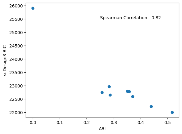
After the simulations, we can check the BIC provided by our package and the calculated ARI to evaluate k-means clustering qualities.

import matplotlib.pyplot as plt

../../_images/da7ff71553f74bf8dc7104f533e0cc4a674cadc841b55e122985adb2568200f3.png