Evaluate pseudotime goodness-of-fit

Introduction

In this example, we will show how to use scDesign3Py to evaluate the pseudotime goodness-of-fit for different pseudotime labels. If the true labels are unavailable and we have little prior knowledge, the scDesign3 BIC can serve as an unsupervised metric. In this tutorial, we will first use the ground truth “pseudotime” generated by the R package dyngen. Then, we will perturb the ground truth pseudotime to worsen its quality and use scDesign3’s BIC to examine pseudotime goodness-of-fit.

Import packages and Read in data

import pacakges

import anndata as ad
import numpy as np
import pandas as pd
import scDesign3Py

Read in data

The raw data is from the R package dyngen. Here, we directly use the result from the scDesign3 tutorial.

data = ad.read_h5ad("data/dyngen.h5ad")

data

AnnData object with n_obs × n_vars = 500 × 155
    obs: 'step_ix', 'simulation_i', 'sim_time', 'pseudotime'
    var: 'module_id', 'basal', 'burn', 'independence', 'color', 'is_tf', 'is_hk', 'transcription_rate', 'splicing_rate', 'translation_rate', 'mrna_halflife', 'protein_halflife', 'mrna_decay_rate', 'protein_decay_rate', 'max_premrna', 'max_mrna', 'max_protein', 'mol_premrna', 'mol_mrna', 'mol_protein'
    uns: 'traj_dimred_segments', 'traj_milestone_network', 'traj_progressions'
    obsm: 'dimred'
    layers: 'counts_protein', 'counts_spliced', 'counts_unspliced', 'logcounts'

Simulation

We perturb the pseudotime by generating random numbers from uniform distribution and replacing various percentages of the original pseudotime with random numbers. The percentage ranges from 0% to 100%. In the code below, we generate 11 sets of perturbed pseudotime with the percentage of perturbation ranging from 0% to 100%. For each new set of perturbed pseudotime, we create a new AnnData object, storing the original count matrix and the corresponding perturbed pseudotime.

perturb_data_dict = {0:{"dat":data}}

for i in range(1,11):
    tmp_data = data.copy()
    num = round(i/10 * len(tmp_data))
    np.random.seed(i)
    tmp_data.obs.loc[tmp_data.obs.sample(n=num,random_state=i).index,"pseudotime"] = np.random.uniform(size=num)
    perturb_data_dict[i] = {"dat":tmp_data}

Then we run scDesign3Py to get the model bic.

for key, value in perturb_data_dict.items():
    tmp_data = value["dat"]
    
    test = scDesign3Py.scDesign3(n_cores=2, parallelization="pbmcmapply")
    test.set_r_random_seed(123)
    res = test.scdesign3(anndata=tmp_data, 
                        pseudotime="pseudotime",
                        corr_formula = "ind", 
                        mu_formula = "s(pseudotime, bs = 'cr', k = 10)", 
                        sigma_formula = "1", 
                        copula = "gaussian", 
                        default_assay_name = "counts", 
                        family_use = "nb",
                        usebam = False)
    
    perturb_data_dict[key]["bic"] = res["model_bic"]

Visualization

After the simulations, we use BIC, which is an unsupervised metric, for evaluating the goodness-of-fit of the pseudotime.

bic_res = pd.concat([i["bic"] for _,i in perturb_data_dict.items()],axis=1).T
bic_res.index = [f"{i/10} perturb" for i in bic_res.index]
bic_res

	bic.marginal	bic.total
0.0 perturb	440744.638950	440744.638950
0.1 perturb	465098.582392	465098.582392
0.2 perturb	471527.503356	471527.503356
0.3 perturb	487017.888671	487017.888671
0.4 perturb	487621.784061	487621.784061
0.5 perturb	493888.709002	493888.709002
0.6 perturb	496339.699622	496339.699622
0.7 perturb	499465.894561	499465.894561
0.8 perturb	499858.520011	499858.520011
0.9 perturb	501529.672888	501529.672888
1.0 perturb	502280.653546	502280.653546

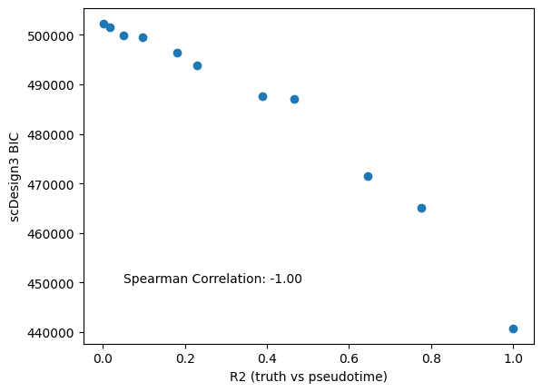
Since we also have the ground truth pseudotime, we also calculate the \(r^2\) between the ground truth pseudotime and perturbed pseudotime. The \(r^2\) is a supervised metric to evaluate the pseudotime qualities. The figure shows that model BICs agree with \(r^2\)

import matplotlib.pyplot as plt

r = []
for i in range(0,11):
    r.append(perturb_data_dict[i]["dat"].obs["pseudotime"].corr(perturb_data_dict[0]["dat"].obs["pseudotime"],"pearson"))
r2 = [i*i for i in r]

../../_images/f2ef2a20fa973d829a2c956f9b14b3a263bf0d583c93f4be6d73320b1536c915.png