Simulate single-cell ATAC-seq data

Introduction

In this example, we show how to use scDesign3Py to simulate the peak by cell matrix of scATAC-seq data.

Import packages and Read in data

import pacakges

import anndata as ad
import numpy as np
import pandas as pd
from sklearn.feature_extraction.text import TfidfTransformer
import scDesign3Py

Read in the reference data

The raw data is from the Signac, which is of human peripheral blood mononuclear cells (PBMCs) provided by 10x Genomics. We pre-select the differentially accessible peaks between clusters. The data was converted to .h5ad file using the R package sceasy.

To save time, we subset 1000 cells and 100 genes

data = ad.read_h5ad("data/ATAC.h5ad")
data = data[data.obs.sample(1000, random_state=123).index,0:100]
data

View of AnnData object with n_obs × n_vars = 1000 × 100
    obs: 'nCount_peaks', 'nFeature_peaks', 'total', 'duplicate', 'chimeric', 'unmapped', 'lowmapq', 'mitochondrial', 'passed_filters', 'cell_id', 'TSS_fragments', 'DNase_sensitive_region_fragments', 'enhancer_region_fragments', 'promoter_region_fragments', 'on_target_fragments', 'blacklist_region_fragments', 'peak_region_fragments', 'nucleosome_signal', 'nucleosome_percentile', 'TSS.enrichment', 'TSS.percentile', 'pct_reads_in_peaks', 'blacklist_ratio', 'peaks_snn_res.0.8', 'seurat_clusters', 'ident', 'cell_type'
    var: 'name'
    obsm: 'X_lsi', 'X_umap'

Simulation

Here we choose the Zero-inflated Poisson (ZIP) as the distribution due to its good empirical performance. Users may explore other distributions (Poisson, NB, ZINB) since there is no conclusion on the best distribution of ATAC-seq.

test = scDesign3Py.scDesign3(n_cores=3,parallelization="pbmcmapply")
test.set_r_random_seed(123)
simu_res = test.scdesign3(
    anndata=data,
    default_assay_name="counts",
    celltype="cell_type",
    mu_formula="cell_type",
    sigma_formula="1",
    family_use="zip",
    usebam=False,
    corr_formula="cell_type",
    copula="gaussian",
)

We also run the TF-IDF transformation.

tfidf = TfidfTransformer()
org_tfidf = tfidf.fit_transform(data.X)
simu_tfidf = tfidf.fit_transform(simu_res["new_count"])

Then we can construct new data using the simulated count matrix and add the tfidf layer.

simu_data = ad.AnnData(X=simu_res["new_count"], obs=simu_res["new_covariate"], layers={"tfidf": simu_tfidf})
data.layers["tfidf"] = org_tfidf

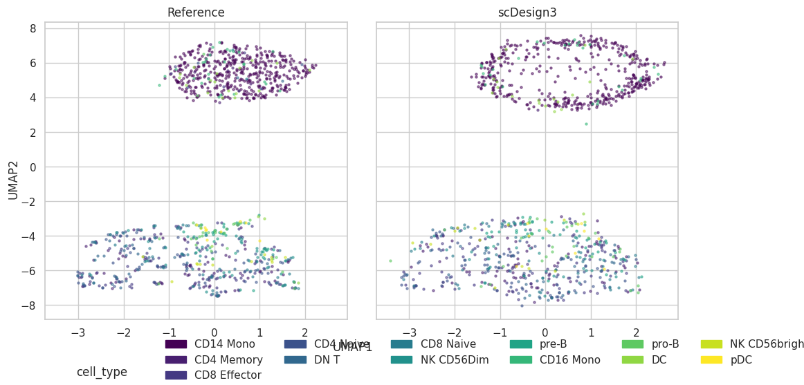
Visualization

plot = scDesign3Py.plot_reduceddim(
    ref_anndata=data,
    anndata_list=simu_data,
    name_list=["Reference", "scDesign3"],
    assay_use="tfidf",
    if_plot=True,
    color_by="cell_type",
    n_pc=20,
    point_size=5,
)

plot["p_umap"]