Simulate multi-omics data from single-omic data

Introduction

In this example, we show how to use scDesign3Py to simulate multi-omics (RNA expression + DNA methylation) data by learning from real data that only have a single modality. The example data and aligned low-dimensional embeddings are from Pamona.

Import packages and Read in data

import pacakges

import anndata as ad
import pandas as pd
import scDesign3Py
import scanpy as sc

Read in the reference data

meth_exp = ad.read_h5ad("data/SCGEMMETH.h5ad")
rna_exp = ad.read_h5ad("data/SCGEMRNA.h5ad")

Simulation

We first use the step-by-step functions to fit genes’ marginal models, copulas, and extract simulation parameters separately for the scRNA-seq data and the DNA methylation data.

rna = scDesign3Py.scDesign3(n_cores=1,parallelization="mcmapply")
rna_data = rna.construct_data(
    anndata=rna_exp,
    default_assay_name="logcounts",
    celltype="cell_type",
    spatial=["UMAP1_integrated","UMAP2_integrated"],
    corr_formula="1"
)

meth = scDesign3Py.scDesign3(n_cores=1,parallelization="mcmapply")
meth_data = meth.construct_data(
    anndata=meth_exp,
    default_assay_name="counts",
    celltype="cell_type",
    spatial=["UMAP1_integrated", "UMAP2_integrated"],
    corr_formula="1",
)

Note here we actually treat the 2D aligned UMAPs as a kind of “pseudo”-spatial data. We use the tensor regression spline to fit two ref datasets seperately.

rna.set_r_random_seed(123)
rna_marginal = rna.fit_marginal(
    mu_formula="te(UMAP1_integrated, UMAP2_integrated, bs = 'cr', k = 10)",
    sigma_formula="te(UMAP1_integrated, UMAP2_integrated, bs = 'cr', k = 5)",
    family_use="gaussian",
    usebam=False,
)

meth.set_r_random_seed(123)
meth_marginal = meth.fit_marginal(
    mu_formula="te(UMAP1_integrated, UMAP2_integrated, bs = 'cr', k = 10)",
    sigma_formula="1",
    family_use="binomial",
    usebam=False,
)

rna_copula = rna.fit_copula(copula="vine")

meth_copula = meth.fit_copula(copula="vine")

rna_para = rna.extract_para(new_covariate=pd.concat([rna_data["dat"], meth_data["dat"]], axis=0))

meth_para = meth.extract_para(new_covariate=pd.concat([rna_data["dat"], meth_data["dat"]], axis=0))

Then, we combined the cell covariates from both the scRNA-seq data and the DNA methylation data as the new covariate to simulate the two new datasets with parameters from scRNA-seq data and the DNA methylation data separately.

rna_res = rna.simu_new(new_covariate=pd.concat([rna_data["dat"], meth_data["dat"]], axis=0),
                       important_feature=rna_copula["important_feature"],)

meth_res = meth.simu_new(new_covariate=pd.concat([rna_data["dat"], meth_data["dat"]], axis=0),
                         important_feature=meth_copula["important_feature"],)

Visualization

We combine the two synthetic datasets and obtain the UMAP embeddings for the combined dataset.

count_combine = pd.concat([rna_res,meth_res], axis=1)
combine_exp = ad.AnnData(X=count_combine)

sc.tl.pca(combine_exp, n_comps=5)
sc.pp.neighbors(combine_exp, n_neighbors=30, n_pcs=5)
sc.tl.umap(combine_exp, min_dist=0.7)

rna_exp.obsm["cov"] = rna_exp.obs.iloc[:,0:5]
sc.pp.neighbors(rna_exp, n_neighbors=30, use_rep="cov")
sc.tl.umap(rna_exp, min_dist=0.7)

meth_exp.obsm["cov"] = meth_exp.obs.iloc[:,0:5]
sc.pp.neighbors(meth_exp, n_neighbors=30, use_rep="cov")
sc.tl.umap(meth_exp, min_dist=0.7)

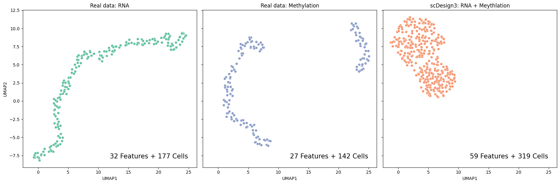
Then we visualize the UMAP embeddings for the inputted scRNA-seq data, DNA methylation data, and the combined synthetic data.

import matplotlib.pyplot as plt
import seaborn as sns

../../_images/f3e8f1a8106ca70de251e49169d9cdf403a53602475391a9b78cd1d2c83b57c7.png