Simulate datasets with cell library size

Introduction

In this example, we will show how to use scDesign3Py to simulate datasets adjusted by cell library size. The purpose of this example is to show that including the library size when modeling the marginal distribution for each gene can help cells in the synthetic data have more similar library sizes as the cells in the real data.

Import packages and Read in data

import pacakges

import anndata as ad
import numpy as np
import pandas as pd
import scanpy as sc
import scDesign3Py

Read in the reference data

The raw data is from the R package DuoClustering2018 which contain a set of datasets with true cell type labels and converted to .h5ad file using the R package sceasy.

data = ad.read_h5ad("data/Zhengmix4eq.h5ad")
data.obs["cell_type"] = data.obs["phenoid"]
data.obs["cell_type"] = data.obs["cell_type"].astype("category")

We then calculate the library size for each cell.

sc.pp.calculate_qc_metrics(data,inplace=True)
data.obs.rename(columns={'total_counts':'library'},inplace=True)

data

AnnData object with n_obs × n_vars = 3555 × 1556
    obs: 'barcode', 'phenoid', 'total_features', 'log10_total_features', 'library', 'log10_total_counts', 'pct_counts_top_50_features', 'pct_counts_top_100_features', 'pct_counts_top_200_features', 'pct_counts_top_500_features', 'sizeFactor', 'cell_type', 'n_genes_by_counts', 'log1p_n_genes_by_counts', 'log1p_total_counts', 'pct_counts_in_top_50_genes', 'pct_counts_in_top_100_genes', 'pct_counts_in_top_200_genes', 'pct_counts_in_top_500_genes'
    var: 'id', 'symbol', 'mean_counts', 'log10_mean_counts', 'rank_counts', 'n_cells_counts', 'pct_dropout_counts', 'total_counts', 'log10_total_counts', 'n_cells_by_counts', 'log1p_mean_counts', 'pct_dropout_by_counts', 'log1p_total_counts'
    obsm: 'X_pca', 'X_tsne'
    layers: 'logcounts', 'normcounts'

Simulation

Then, we set the mu_formula as cell_type and offsetted by the cell library size to generate new dataset adjusted by library size. The library size is log-transformed because the link function for \(\mu\) of the negative binomial distribution in GAMLSS is log.

test = scDesign3Py.scDesign3(n_cores=3,parallelization="pbmcmapply")
test.set_r_random_seed(123)
simu_res = test.scdesign3(    
    anndata = data,
    default_assay_name = "counts",
    celltype = "cell_type",
    other_covariates = "library",
    mu_formula = "cell_type + offset(log(library))",
    sigma_formula = "1",
    family_use = "nb",
    usebam = False,
    corr_formula = "1",
    copula = "gaussian",
    important_feature = "auto")

Then we can construct new data using the simulated count matrix.

simu_data = ad.AnnData(X=simu_res["new_count"], obs=simu_res["new_covariate"])
simu_data.layers["log_transformed"] = np.log1p(simu_data.X)
data.layers["log_transformed"] = np.log1p(data.X)

Visualization

import matplotlib.pyplot as plt
import seaborn as sns

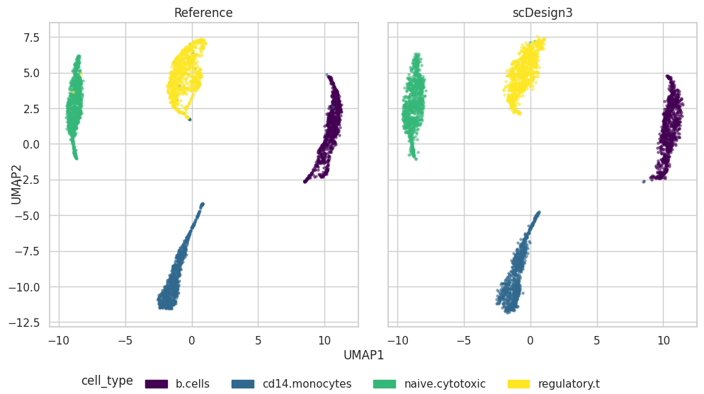
plot = scDesign3Py.plot_reduceddim(
    ref_anndata=data,
    anndata_list=simu_data,
    name_list=["Reference", "scDesign3"],
    assay_use="log_transformed",
    if_plot=True,
    color_by="cell_type",
    n_pc=20,
    point_size=5,
)

plot["p_umap"]

../../_images/c7e1b62a10230361e7c612fa1f1ce7734e8efb862e04bbbe563c7e0f4e9969fa.png

The violin plot below shows the cells in simulated dataset have similar library size as the cells in the reference dataset.

../../_images/641c53e6f9e7ea23ac79d457633366a806f7dfd8ea66023e0e73c3bc3bc98268.png